
3D visualization of astronomical data using Pyvista
This project was done during 5.2021-9.2021 at the Department of Computer Scince at Aalto University in the Astroinformatics group.
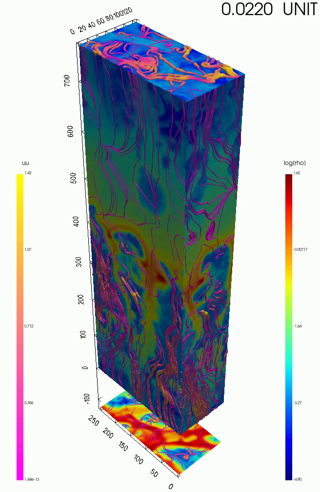
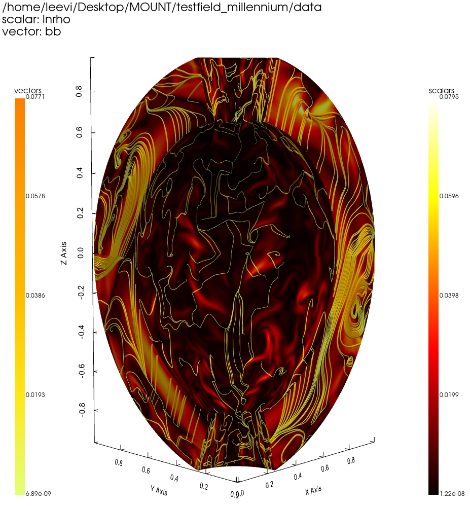
Aim of this work was to create visualizations for 3D astronomical data. This includes both scalar and vector fields. The data itself consisted of either volumetric data or 4x 2D slices from a volume. These four slices are along each of the axes of the coordinate system (with one extra slice). In the case of cartesian coordinates these slices could then be assembled into a box for visualization purposes (shown on the right).
The astronomical simulation data itself comes from the pencil-code simulations and was visualized using Pyvista. Most of the visualizations were run locally though longer movies were generated on the CSC Puhti supercomputing cluster. The developed code itself can also be found from the
Some of the implemented features include:
-
Visualizations in different coordinate systems: cartesian / spherical / cylinder
-
Creating videos from time-series scalar and vector field data (see video demos below, first video)
-
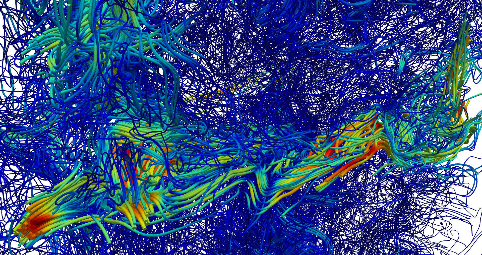
Different methods of vector field visualization: streamlines / vector arrows, colormapping these and scaling according to vector magnitude
-
Other visualization methods including volume rendering of scalar volumetric data, plotting isovalues and different interactive methods of data visualization (e.g. an interactively controlled slicing plane).
Some sample nice sample visualizations are shown in the next gallery. The two first isovalue visualizations are gifs showing a moving range of isosurfaces of a scalar field. The images / gifs might take a moment to load fully.
Video demos
Here are a few example demo videos I had generated using the developed plotting utilities. Unfortunately the quality seems bad after uploading and in addition the starting aspect ratio is a bit awkward (something to fix?). Note that for the latter two of the videos the playback speed has been doubled or tripled.
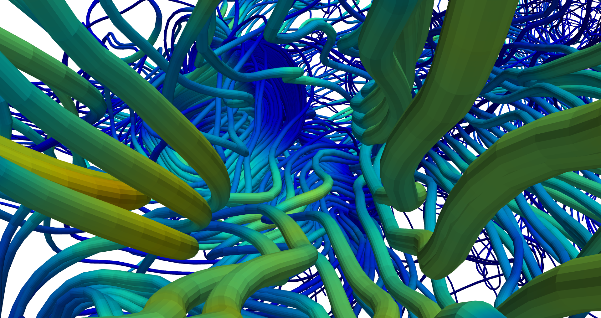
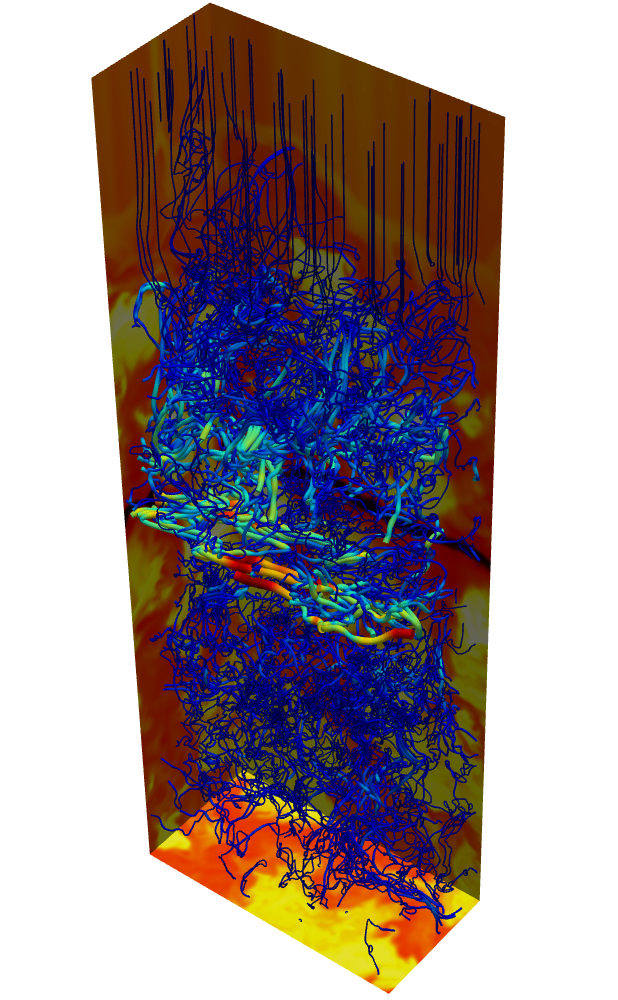
- First video shows the time-evolution of velocity (left) and magnetic fields (right). These are visualized using streamlines - colormap and stream radius scaling shows the magnitude of the field at a point. Below streamlines the colormap shows the logarithmic density $\log\rho$.
- Second video shows a volume rendering of scalar volumetric data (density). In addition the vector field (velocity) is shown by the streamlines in the volume. This is an interactive window that is opened by the plotting script and the slider controls the opacity of the volume rendering.
- And finally the third video shows an interactive slice widget* where one can control the location and orientation of a slicing plane. With this one can see more clearly the behaviour of the scalar and vector fields inside a volume without other data obstructing the view.